
WP3 Multi-wavelength solar image processing for novel SSI proxies
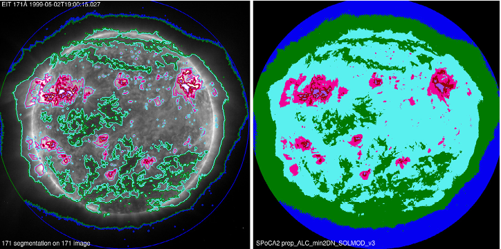
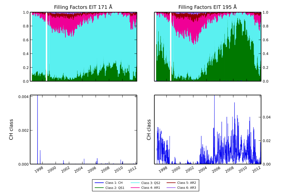
1) EUV image segmentation
Further Reading
2) Image segmentation with the ASAP tool
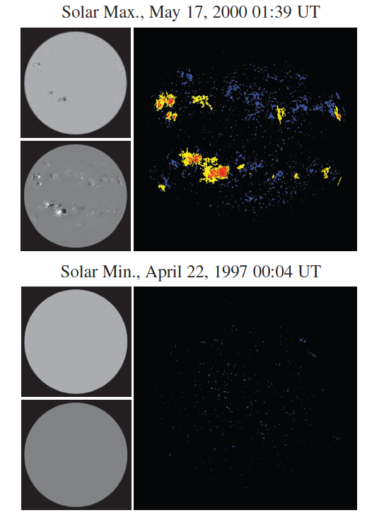
Figure 3: The left panels shows the original MDI intensitygram (top) and magnetogram (bottom). The right panels shows a colour map of the detected solar features: umbra (red), penumbra (orange), faculae (yellow), and network (blue); from Ashamari et al. (2015)
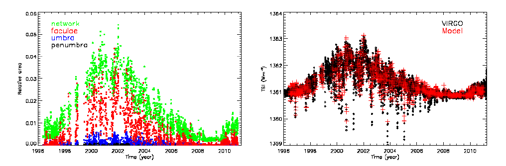
Figure 4: The left panel gives the relative area of the full solar disk of network (green), faculae (red), umbra (blue), and penumbra (black). The right panel compares the fitted TSI data (red) with the VIRGO data corrected to the SI-scale (black); from Ashamari et al. (2015).
Further Reading
3) Ground-based image segmentation
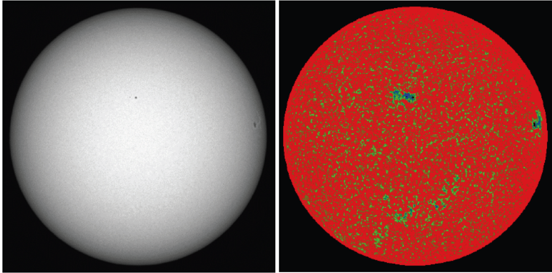
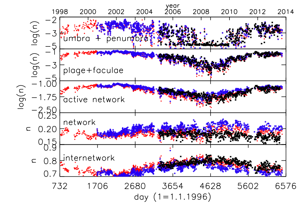
Figure 5: Top left: sample Blue Continuum PSPT image. Right: corresponding mask of features identified with SRPM. Orange: quiet sun; dark green: network; light green: enhanced network; light blue: plage; dark blue: bright plage/faculae; black: sunspot penumbra; dark red: sunspot umbra. Bottom: time dependent area coverage of the various features.
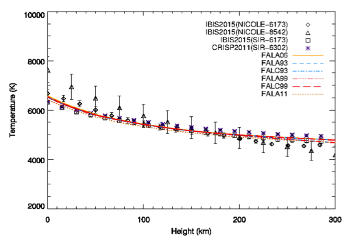
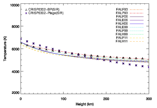
Figure 6: Left panel: Temperature profiles in the quiet Sun subFoVs as a function of height in the formation layers of the Fe I lines. Different symbols correspond to the different datasets used, lines correspond to the different models employed for comparison. Right panel: Temperature profiles in active network regions as a function of height in the formation layers of the Fe I lines. Different symbols correspond to the different datasets used, solid lines corresponds to the models employed for comparison (see Christaldini et al., 2016).
The following Deliverables will be provided within WP3:
D3.1) Filling factors catalogue for SOHO magnetogram and continuum images [month 8]
D3.2) Filling factors catalogue for SOHO EUV images [month 8]
D3.3) Filling factors catalogue for ground-based images [month 18]
D3.4) Filling factors catalogue for PROBA2 images [month 23]
D3.5) Filling factors catalogue for PICARD images [month 26]
D3.6) Higher level SSI products: Provision of higher level products by inter-calibrating the proxies produced inprevious tasks [month 29]
D3.7) Compilation of segmentation maps into SOTERIA Data Archive [month 23]